Prior Partners in Progress reports have described our work in establishing a robust high-throughput system for collecting wheat field imagery and processing this imagery into geo-referenced, plot-level images (see Unmanned Aerial Systems-Based High-Throughout Phenotyping 2023 and Evaluating Image Processing Methods for High-Throughout Phenotyping 2024). In addition to continuing to collect and process imagery data on the OSU Wheat Improvement Team Dual-Purpose Observation Nursery (DPON), work in 2025 focused on building approaches to translate plot-level images into phenotypes that can be used by the research team to select winning wheat varieties. This research can be divided into two main categories: feature engineering and model development. Feature engineering is the process modelers use to identify the properties of a dataset that will best inform model building and the prediction of phenotypes of interest. Model development is specifically the part of the process where we build new models, fit them to the training data we have, and then evaluate the trained models based on independent datasets. We worked on both areas in 2025.

 

Feature Engineering

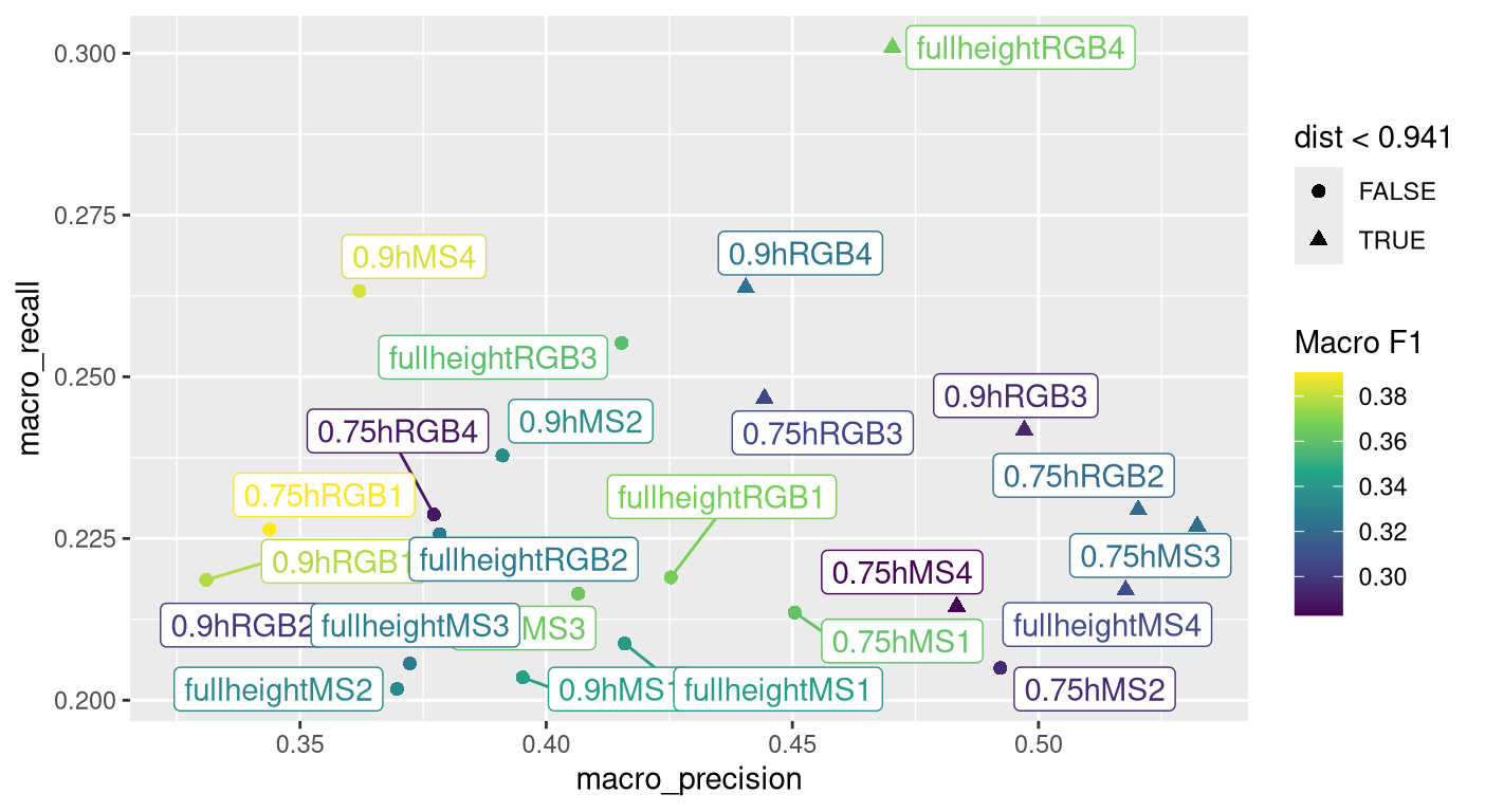
In feature engineering, we are exploring various methods for extracting features of interest from imagery. In the last year, we began an analysis to compare imagery type, plot-level image statistical metrics and plant-height thresholding in terms of their contribution to predicting Barley Yellow Dwarf (BYD) severity scores. For this analysis, we considered two imagery types: visible-spectrum imagery (i.e. red-green-blue; RGB) and multispectral (MS) imagery, which included bands from the visible and beyond the visible spectrum. The plot-level statistical metrics considered in the analysis included different combinations of plot-level mean, standard deviation, skewness and kurtosis. Standard deviation is an overall measure of how similar all pixels of a plot-level image are to the plot-level mean. Skewness is a measure of how much pixel values are concentrated above or below the plot-level mean. Kurtosis measures the proportion of pixel values that are very far above or below the mean. The four combinations we evaluated were only mean (1); mean and standard deviation (2); mean, standard deviation and skewness (3); and all four statistical metrics (4). The three plant-height threshold scenarios we considered for this analysis included summarizing all pixels from a plot (full height), summarizing only pixels above 75% of the plant height for the plot (0.75h) and summarizing only pixels above 90% of the plant height for the plot (0.9h). Figure 1 shows a preliminary analysis that combines three different measures of model performance: macro recall, macro precision and macro F1 (a type of average of recall and precision). Higher is better for all three of these models. The triangles in Figure 1 indicate the best-performing one-third of the 24 feature combinations analyzed in this study. Overall, using imagery from the visible spectrum (RGB) with the maximum number of pixel-level statistics (4) and no height thresholding gave the best prediction of BYD severity. Based on these results, we can provisionally conclude that the addition of all four statistical metrics (mean, standard deviation, skewness, and kurtosis) helped us capture subtle within-plot variations, which improved prediction over the conventional approach of using simple plot-level means for modeling.

 

Figure 1. Diagram showing model metrics for 24 combinations of imagery type with macro-recall on y-axis, macro-precision on x-axis and color filled with macro-F1 values. Higher values are better for all model metrics. Triangles indicate combinations performing in the top third in predicting barley yellow dwarf disease severity.

 

Model Development

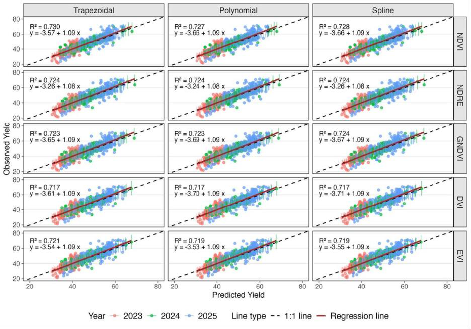
In the area of model development, we are exploring two main types of modeling approaches. The first approach is statistical modeling based on non-linear regression. Our team tested three non-linear regression models to analyze the data using multispectral imagery, including trapezoidal, polynomial and splines. The trapezoidal model essentially used straight lines to connect measurements for each plot over the growing season. The polynomial model fit a single curve across all measurement dates. The splines model fit multiple curves over subsets of neighboring measurement dates. All three models were then used to calculate the area under the curve to generate a measure of the amount of time the crop had a full, healthy canopy. We evaluated these models in the context of five different vegetative indices (NDVI, NDRE, GNDVI, DVI, EVI). Figure 2 illustrates the accuracy of our predictions (horizontal axis) in matching the actual harvested yield (vertical axis) across three growing seasons (2023-2025) for various wheat varieties. The fact that the colored dots, each representing a different wheat plot, line up closely along the solid red line indicates that our predictions are quite accurate, explaining approximately 72% to 73% of the variation in final yield. We found that all methods yielded nearly identical results, effectively predicting the final wheat yield across various years and growing conditions. This suggests that the simpler trapezoidal modeling approach can be used without compromising accuracy in model predictions.

 

Figure 2. Observed versus predicted wheat yield across methods and vegetation indices. R2 values close to 1 indicate a good fit.

 

A second approach to modeling that we are exploring relies on process-based crop modeling. This type of model mimics the behavior of the crop using equations for processes, such as photosynthesis, respiration and crop development. These equations are linked together into a computer model that can be used to simulate the growth and development of a crop as affected by weather, soil and management from day to day over a whole growing season from planting to harvest. 

 

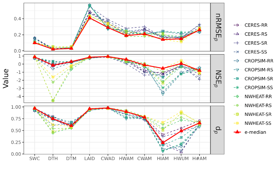
For this modeling approach, we trained a set of existing process-based wheat models for a single genotype and evaluated their performance using three different statistical metrics across a wide range of available crop data variables (Figure 3). We also considered the performance of the median of the full set (ensemble) of wheat models (e-median). Overall, the ranges of values shown by different wheat models and the e-median were within acceptable ranges for different types of winter wheat data as reported in prior studies. Although not a single wheat model performed best for all the data variables, the e-median performed better than the best performing model for nearly all variables. This suggests that using an ensemble of models may be a better strategy for more accurate prediction than relying on any single model. Additionally, this study provided a set of well-calibrated and validated wheat crop models for Oklahoma wheat regions, which can be used for other studies. Future work in this area will evaluate process-based modeling linked with wheat imagery for generating model-derived phenotypes that can be used for future selection.

 

Figure 3. Predictive performance of a collection (ensemble) of process-based crop models and the median of the overall ensemble (e-median) for soil water content (SWC), days to heading (DTH), days to maturity (DTM), in-season leaf area index (LAID), in-season biomass (CWAD), end-season biomass (CWAM), grain yield at maturity (HWAM), harvest index at maturity (HIAM), individual grain weight at maturity (HWUM), and number of grains per meter square at maturity (H#AM) assessed with three different statistical metrics: normalized root mean squared error (nRMSE_p), Nash–Sutcliffe efficiency (NSE_p) and Willmott agreement index (d_p). For nRMSE_p, values closer to zero are better. For NSE_p and d_p, values closer to one are better.